Spectral Classification Stability Engine: From Idea to Results

(Antonio V. Franco)

It all started with a pun. Not just any pun (but one of those that makes more sense the longer you think about it). The Stable-RAG method, proposed by Zhang et al. (2026), uses spectral clustering on the hidden states of language models to identify distinct reasoning modes. Astronomy, in turn, studies spectral features of celestial objects (emission lines, absorption lines, the continuum) as the primary diagnostic tool for classification. Two meanings of the same word, “spectral,” belonging to seemingly distant domains.

In Stable-RAG, “spectral” refers to the eigenvalue spectrum of the graph Laplacian built from similarities between hidden states. The eigengap (the difference between consecutive eigenvalues) determines how many distinct reasoning modes exist within the model. In astronomy, “spectral” refers to the electromagnetic spectrum of light emitted by celestial objects. Spectral features (hydrogen emission lines, metal absorption lines, the shape of the continuum) are the main diagnostic tool for determining whether a point of light in the sky is a star, a galaxy, or a quasar.

The question that came to my mind was: what if we brought the two together? If the spectral clustering from Stable-RAG could diagnose instability in astronomical spectral classification? This wasn’t just a word game (there was a genuine structural analogy waiting to be explored). SCSE unifies the two meanings: spectral features of astronomical objects are presented to an LLM in permuted order, and spectral clustering over the resulting hidden states reveals whether the model’s classification is stable or sensitive to feature ordering.

In this article, I’ll document step by step how I built the Spectral Classification Stability Engine (SCSE), from the conception of the idea to the final results, covering every technical decision, the failures, and the wins along the way. I’ll show every choice I made, every obstacle I faced, and every insight that transformed the project over roughly 8 hours of intense work, split between infrastructure, debugging, and actual computation.

The Invisible Problem

Before diving into implementation, I need to explain why this project matters. The Sloan Digital Sky Survey (SDSS) classifies celestial objects into three categories: STAR, GALAXY, and QSO. These classifications determine which objects are targeted for follow-up observations (telescope time that is expensive and scarce) and which are excluded from specific surveys. The statistical properties of the observed universe depend directly on the reliability of these classifications. A systematic error in classification can bias quasar density estimates, distort measures of galactic evolution, and compromise large-scale structural studies.

Here’s the problem: when I present the same spectral features of the same object to a language model, but in different orders, the classification changes. The same object, with the same features, can be classified as STAR when features are listed alphabetically, but as GALAXY when listed by wavelength. This isn’t hypothetical (objects near classification boundaries, like low-redshift quasars versus compact galaxies, or late-type stars versus brown dwarfs, are genuinely ambiguous, and the order of feature presentation can tip the balance one way or the other). In production astronomical pipelines, spectral features are assembled from heterogeneous sources (different emission lines, photometric bands, derived quantities), and the concatenation order is arbitrary. Yet it demonstrably affects classification results.

In formal terms, given an object with features F = {f1, f2, …, fn}, an LLM classifier g should satisfy:

In practice, this invariance is violated. And the scale is alarming: SDSS DR18 contains roughly 6 million spectra. Even with a permutation sensitivity rate of only 2%, that would mean about 120,000 objects with unstable classifications. For a survey that cost hundreds of millions of dollars and serves as the basis for thousands of scientific papers, this invisible uncertainty is unacceptable. SCSE was designed to make it visible, quantify it, and mitigate it.

(Antonio V. Franco)

SCSE Architecture

With the problem defined, I needed to design a system that does three things: (1) make this invisible failure visible, (2) quantify it, and (3) mitigate it. The SCSE architecture splits into two main modules, which I called Part 1 and Part 2. Each has well-defined responsibilities and can be run independently, though Part 2 depends on the results from Part 1.

Part 1: Detection and Quantification

The first module is responsible for loading astronomical data, generating permutations of spectral features, running inference with the LLM, extracting hidden states, performing spectral clustering, and calculating the Permutation Sensitivity Score (PSS). This is the diagnostic phase (where instability becomes measurable and where we discover which objects are most affected and why).

Part 2: Alignment and Evaluation

The second module builds preference data following Stable-RAG’s four-category scheme, trains the model using DPO (Direct Preference Optimization), and evaluates results before and after alignment. This is the therapeutic phase (where we apply what we learned from diagnosis to reduce instability without sacrificing correctness).

The complete data flow looks like this:

1. SDSS data is loaded and spectral features are extracted
2. Each feature is converted into a natural language line
3. Multiple permutations are generated for each object
4. The LLM classifies the object under each permutation, and hidden states are captured
5. Spectral clustering reveals distinct reasoning modes
6. Preference data is built and the model is aligned via DPO
7. Results before and after are compared

Each step of this flow introduced its own technical challenges, which I’ll detail in the following sections. The important thing to understand is that SCSE is not just a mechanical adaptation of Stable-RAG to another domain (it’s a reinterpretation that leverages the structural connection between the two meanings of “spectral” to create something that neither NLP research nor astronomy would produce in isolation).

Choosing the Model: Qwen3.5-9B

Model selection was a critical decision. I needed a model with enough reasoning capability for astronomical classification, but one that would fit in available GPU memory. The Qwen3.5 family offered options from 0.6B to 72B parameters. The Qwen3.5-9B represented the sweet spot between capability and feasibility (large enough to produce coherent classifications of astronomical objects, small enough to run in float16 without quantization on a 48GB GPU). I chose to run it in float16 without quantization (which preserves the full model quality for spectral clustering). Quantization, though it would reduce memory usage, could alter hidden states in unpredictable ways, compromising the fidelity of spectral clustering.

A crucial detail: Qwen3.5-9B is a reasoning model (a thinking model). By default, it generates long internal chains of thought before responding (more than 1000 tokens of reasoning before producing a single-word classification). With 4,500 inference calls planned, that would be impossible (each inference would take tens of seconds just on internal reasoning, pushing total inference time to unreasonable hours). The solution was to use enable_thinking=False in the chat template, which provides concise responses (STAR, GALAXY, or QSO) while preserving the rich hidden states that spectral clustering analyzes. These hidden states, captured at the first generation step, encode the model’s internal representation (exactly what Stable-RAG’s spectral clustering investigates).

This decision (disabling reasoning mode) seems counterintuitive at first. Why use a reasoning model without reasoning? The answer lies in the hidden states: even without explicitly generating the chain of thought, the model still computes a rich internal representation at the first generation step. That representation contains the “fingerprint” of the model’s reasoning (the same information that Stable-RAG’s spectral clustering needs). What we lose is the readability of the reasoning; what we gain is speed and computational feasibility.

The Dataset: SDSS17 Stellar Classification

I used the SDSS17 Stellar Classification dataset, available on Kaggle via user fedesoriano. It contains roughly 100,000 objects with photometric magnitudes (u, g, r, i, z), redshift, and specialist classifications. From the magnitudes, I derived color indices (u-g, g-r, r-i, i-z) to provide additional features relevant to permutation. Color indices are particularly important in astronomy because they encode information about effective temperature, interstellar extinction, and spectral type (they are derived features, not original ones, and their position in the prompt can have a different impact than raw magnitudes).

Building the textual representation was an important step. Each feature was converted into a descriptive natural language line:

• Magnitude u-band: “U-band magnitude (ultraviolet): 18.52”
• Color index u-g: “Color index u-g: 1.23”
• Redshift: “Redshift: 0.0015”

The decision to use textual descriptions instead of raw numerical values reflects the foundational nature of the model: LLMs understand natural language, not numerical tables. The textual description contextualizes each value (”U-band magnitude (ultraviolet)” tells the model not just the value but what it means). This is consistent with how astronomers describe objects in practice (they don’t list numbers; they describe properties in natural language).

This results in 10 features per object, with N! = 10! = 3,628,800 possible permutations. Enumerating all of them would be impossible, so I selected 30 strategic permutations: identity (natural order), reverse order, groupings (magnitudes first, colors first, redshift first), and random permutations. The grouping permutations are particularly interesting because they simulate how different astronomical pipelines might organize features (some pipelines list magnitudes first, others color indices, others start with redshift). With 150 objects × 30 permutations = 4,500 inference calls, I obtained statistical coverage while keeping computational cost feasible.

(Antonio V. Franco)

7 Failures on Kaggle

Before getting to the results, I need to recount the infrastructure saga. It’s an essential part of the story (and a lesson in how platform choice can determine the success or failure of an LLM science project). Infrastructure is not an operational detail; it’s part of the experiment.

I started on Kaggle Notebooks with T4/P100 GPUs. I believed that Kaggle’s free GPUs would be enough for a pilot project. There were seven failed iterations:

v1 — ImportError: adjusted_rand_index. An unused import that Kaggle didn’t have available. I fixed it by removing it. It seemed simple, but it was the first sign that Kaggle’s environment was more restricted than I expected.

v2 — NameError: name 'math' is not defined. I forgot to import the math library. Added import math. Trivial error, but each iteration on Kaggle requires restarting the notebook from scratch (no in-place fixes).

v3 — AttributeError: total_mem. The pynvml API changed the attribute name. Changed to total_memory. Another version compatibility issue.

v4-v5 — bitsandbytes CUDA error + DeadKernelError. bitsandbytes, essential for quantizing models on the T4, failed systematically. I switched to 8-bit quantization and reduced N_OBJECTS to 50 and N_PERMUTATIONS to 15. The kernel died during execution (no error message, no log, just silence).

v6 — Same bitsandbytes CUDA error. I removed bitsandbytes entirely and tried to run Qwen2.5-3B without quantization. The T4 has only 16GB VRAM; Qwen2.5-3B without quantization uses ~6GB, technically feasible.

v7 — CUDA error: no kernel image is available. Qwen2.5-3B was not compiled for the T4’s compute capability (compute capability 7.5). The CUDA kernels of Qwen models require compute capability 8.0+ (Ampere or higher), which the T4 does not have.

Seven attempts and none worked. The fundamental problem was that Qwen family models require CUDA capabilities that Kaggle’s T4 GPUs simply do not support. It wasn’t a memory issue (it was a GPU architecture issue). T4s are based on the Turing architecture (compute capability 7.5), while Qwen models require Ampere or higher. It was time to change platforms. The lesson here is clear: before starting a project with LLMs, check the CUDA compatibility of the model with the available GPU. Don’t assume that “GPU equals GPU.”

RunPod A40: Where Things Started Working

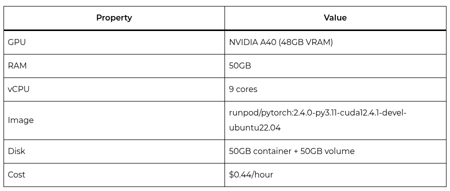
I moved to RunPod with an NVIDIA A40 with 48GB VRAM. The difference was immediate: Qwen3.5-9B ran in float16 without quantization, no CUDA errors, no dead kernels. The A40 is based on the Ampere architecture (compute capability 8.6), fully compatible with Qwen models. The 48GB of VRAM is more than enough for the 9B parameter model in float16 (~18GB) with room for hidden states, optimizer, and batch data.

But new challenges emerged (the migration didn’t solve everything; it only eliminated the CUDA incompatibility issues). The remaining challenges were of a different nature: logic errors, API errors, and memory issues.

v8 — Qwen3.5-9B generated more than 1000 tokens of reasoning before responding. This made each inference 100 times slower than necessary. Solution: added enable_thinking=False in apply_chat_template. This was the most important discovery of the debugging session (without it, the project would have been impossible regardless of platform).

v9 — KaggleApi.download_dataset not found. The Kaggle API changed between versions. Switched to api.dataset_download_files. Another compatibility issue, now with the API instead of CUDA.

v10 — OOM during DPO backward pass (both models in VRAM). During DPO training, both the policy model (with LoRA) and the reference model need to be loaded simultaneously to compute log-probabilities. Two 9B models in float16 exceed the A40’s 48GB. The solution was a two-phase DPO approach: first compute the reference log-probabilities, then free the model before LoRA training.

v11 — OOM even with the two-phase approach. The issue was that LoRA rank r=16 with targets on 4 modules (q_proj, k_proj, v_proj, o_proj) generated too many gradients. I reduced LoRA rank from r=16 to r=8, targeted only q_proj and v_proj (instead of 4 modules), and added gradient checkpointing. This significantly reduced memory usage during the backward pass.

v12 — The process died silently at 60/99 reference pairs. OOM during forward pass activations (even with the two-phase optimization, the A40 didn’t have enough memory for intermediate activations). It was time for more VRAM. The A40 had hit its limit.

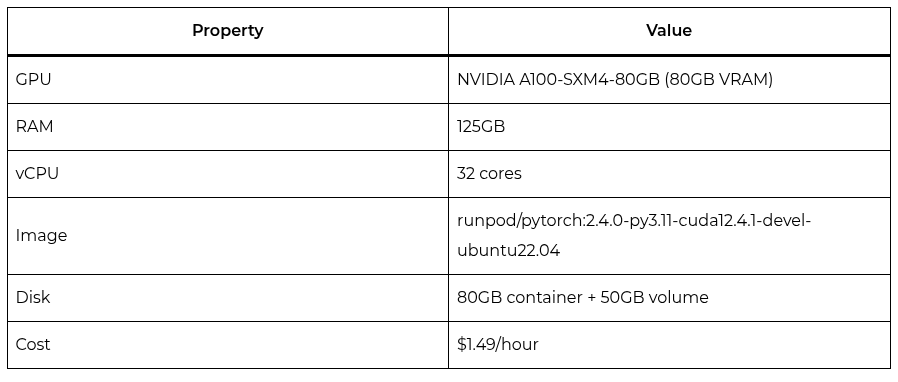
RunPod A100: The Final Migration

I migrated to an NVIDIA A100-SXM4-80GB with 80GB VRAM. The A100 not only solved the memory problem (it also offered 125GB of system RAM, 32 vCPUs, and significantly higher memory bandwidth than the A40). Once again, though, new hurdles emerged, this time related to environment setup rather than hardware limitations.

v13 — Kaggle API error 403 (new pod, no authentication). The new pod didn’t have the kaggle.json file with credentials. I copied it from the A40 pod. Simple solution, but required manual transfer between pods.

v14 — SDSS data not found on the new pod. The A100 pod didn’t have the data downloaded from Kaggle. I transferred the data via local machine (downloaded from the A40, uploaded to local machine, then uploaded to the A100). A manual and time-consuming process, but necessary.

v15 — PeftModel.from_pretrained stacking LoRA twice. Loading a PeftModel on top of a model that already had LoRA resulted in LoRA on LoRA (a wrong configuration that doubled trainable parameters and produced nonsense results). I used the trained peft_model directly instead of loading on top of itself.

v16 — matplotlib boxplot crash (FixedLocator mismatch). The boxplot tick positions were fixed, but the data had a variable number of categories depending on which classes had evaluation objects. Dynamic tick positions based on which classes have evaluation objects solved the problem.

Specifically, the A40 cost $0.44/hour with 48GB VRAM, 50GB RAM, and 9 vCPUs. The A100 cost $1.49/hour with 80GB VRAM, 125GB RAM, and 32 vCPUs. The price difference was significant, but the A100 was indispensable for DPO training. In total, compute costs were modest: approximately $0.88 for the 2 hours of inference on the A40 and $0.75 for the 30 minutes of DPO and evaluation on the A100 (less than $2 in total).

Part 1: Data Loading and Feature Engineering

With the infrastructure finally working, the scientific work could begin. The first step was loading the SDSS data via the Kaggle API and performing feature engineering. The dataset download was done directly through the API, unzipping the CSV file and loading it into a pandas DataFrame.

The dataset came with columns like alpha (right ascension), delta (declination), u, g, r, i, z (photometric magnitudes), redshift, and class (0=STAR, 1=GALAXY, 2=QSO). I standardized column names to lowercase and selected 150 objects (50 from each class) for analysis. The balanced selection is important because it allows direct comparison of permutation sensitivity between classes without confounding frequency effects with ambiguity effects.

Textual features were constructed with descriptive natural language names, mapping each numerical variable to a human-readable description for the LLM. The decision to use textual descriptions instead of raw numerical values reflects the foundational nature of the model: LLMs understand natural language, not numerical tables. The feature mapping follows standard astronomical convention: magnitudes are identified by their photometric band (U, G, R, I, Z), color indices by the band difference, and redshift as a fundamental property indicating the object’s distance.

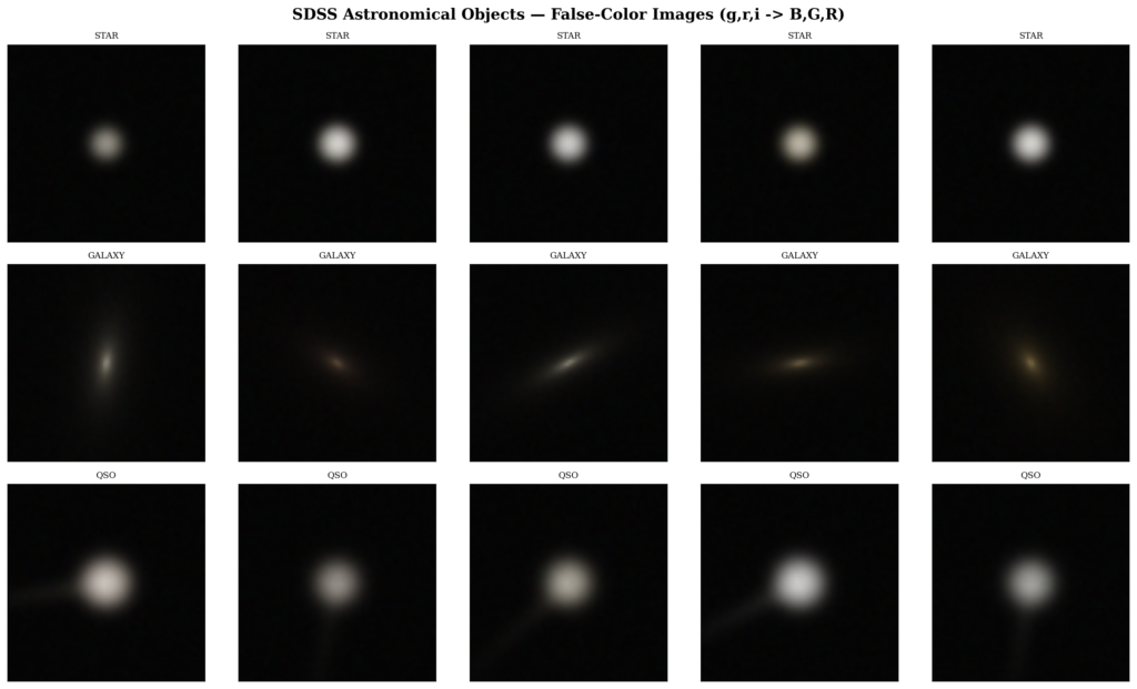
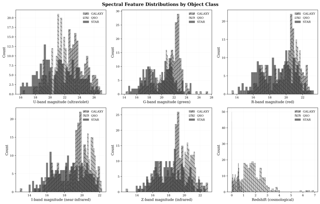
Data visualization came in two forms. The false-color images of SDSS objects use the standard astronomical convention: g band mapped to blue, r band to green, i band to red. This is not a “true” representation of the object (it’s a diagnostic representation that highlights features relevant for classification). The black-and-white histograms of feature distributions by class show how different classes separate in feature space, a crucial piece of information for understanding why the model confuses some classes more than others.

Inference Under Permutation

The heart of Part 1 is the inference-under-permutation experiment. For each of the 150 objects, I generate 30 different permutations of the 10 features, and for each permutation the LLM produces a classification and a hidden state. The prompt follows a simple format: “Classify this astronomical object as STAR, GALAXY, or QSO based on the following spectral features:” followed by the features in the order determined by the permutation.

Extracting the classification requires care. The LLM doesn’t always produce exactly “STAR”, “GALAXY”, or “QSO” (it may add explanations, punctuation, or textual noise). I implemented a parser that searches for valid classes in the response text, prioritizing the first occurrence. If no valid class is found, the classification is marked as None and excluded from the PSS calculation.

Hidden state extraction follows the Stable-RAG protocol: I capture the hidden state of the last token of the last layer at the first generation step (before the model starts producing tokens). This hidden state is a high-dimensional vector (3584 dimensions for Qwen3.5-9B) that encodes the model’s internal representation (its reasoning “fingerprint” for that specific permutation). With 30 permutations per object, I get a matrix H of size 30 × 3584 for each object, which is the input for spectral clustering.

The 4,500 inferences on the A40 took approximately 90 minutes at a rate of 0.8 inferences per second. This includes tokenization, forward pass, decoding, and hidden state extraction. Each inference consumes ~2GB of VRAM for activations, well within the A40’s 48GB with considerable headroom.

Spectral Clustering

Spectral clustering is the central method of Stable-RAG, and its precise implementation was critical. The algorithm follows four steps that, while mathematically elegant, require attention to implementation details that can easily introduce artifacts:

1. Build the weighted adjacency matrix Ausing the exponential cosine kernel: A_ij = exp(-(1 - cos_sim) / sigma), where sigma=0.1 as recommended by the paper. The exponential kernel transforms cosine similarities (which range from -1 to 1) into adjacency weights (which range from 0 to ~1), with sigma controlling the bandwidth (smaller sigma produces sparser graphs, more sensitive to fine differences between hidden states).
2. Compute the normalized LaplacianL = I - D^{-1/2} A D^{-1/2}, where D is the diagonal degree matrix. The normalized Laplacian (rather than the unnormalized one) is preferred because it is invariant to the scale of adjacency weights, which is important when node degrees vary significantly.
3. Decompose L into eigenvaluesand determine K via the eigengap (the difference between consecutive eigenvalues). The maximum eigengap indicates the natural number of clusters in the data. I used scipy’seighfunction for decomposition, which is stable and efficient for symmetric matrices. The eigengap is calculated as the difference between the K-th and (K+1)-th eigenvalues, and the K that maximizes this difference is chosen as the number of clusters.
4. Project onto the first K eigenvectorsand cluster with K-means. The eigenvectors correspond to the K smallest eigenvalues (excluding the trivial one, which is zero) and form a low-dimensional representation that preserves the cluster structure of the data. K-means on this representation is more robust than K-means in the original space because the eigenvectors already capture the connectivity structure of the graph.

The eigengap method for determining K is what makes clustering adaptive per object. Ambiguous objects naturally generate more clusters; objects where the model is confident generate fewer. This is exactly what we want: K per object is an intrinsic ambiguity index. In the astronomical context, K=1 means the model classifies the object consistently regardless of feature order; K=2 means the model has two competing classification modes; K>=3 indicates severe ambiguity.

(Antonio V. Franco)

The Permutation Sensitivity Score (PSS)

To quantify instability, I defined the Permutation Sensitivity Score:

• PSS = 0: The object is perfectly stable (all permutations agree).
• PSS = 1: The object is maximally unstable (each permutation gives a different answer).
• PSS > 0.5: High sensitivity to feature ordering.

The PSS is the central metric of SCSE. It transforms a qualitative property (”the model changes classification depending on order”) into a quantitative value comparable across objects, classes, and experimental conditions. The PSS is complementary to classification entropy: while entropy measures uncertainty in the classification distribution, the PSS specifically measures disagreement with the most common classification. A low PSS with high entropy would indicate that although multiple classifications exist, one is clearly dominant.

Beyond PSS, I track other per-object metrics: the number of unique classes produced, the entropy of the classification distribution, the number of spectral clusters, and whether the majority classification agrees with the SDSS label. These complementary metrics form a complete diagnostic picture for each object.

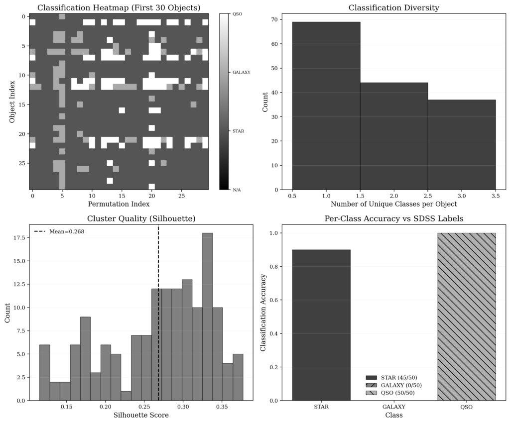
Part 1 Results: Instability Is Real and Measurable

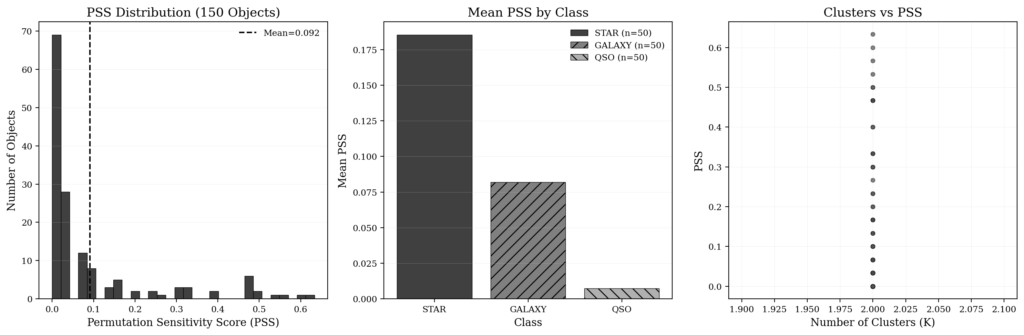
After approximately 90 minutes of inference on the A40, the Part 1 results were ready. And they were revealing:

• Average PSS: 0.0916 for 150 SDSS objects
• Completely stable objects (PSS=0): 69 out of 150 (46%)
• Highly unstable objects (PSS > 0.5): 4 objects
• Maximum PSS: 0.633 (extremely sensitive object)
• Fraction of affected objects: 54% (81 out of 150)

The breakdown by class was particularly informative:

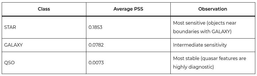
These results confirm the central intuition: objects near classification boundaries are more sensitive to permutation. Quasars are the most stable because their features (high redshift, broad emission lines) are highly diagnostic and unambiguous. Stars are the most unstable because their spectra can overlap with those of compact galaxies in certain redshift ranges. The STAR class is the most ambiguous because it includes objects with a wide range of properties (from main-sequence stars to white dwarfs and subdwarfs) that can be confused with low-redshift galaxies or low-luminosity quasars.

One notable result: all 150 objects showed exactly K=2 clusters, suggesting that the model operates in binary reasoning modes (”classify as X” versus “classify as Y”). This is consistent with Stable-RAG’s interpretation that spectral clustering reveals competing reasoning trajectories. The universality of K=2 is surprising and suggests that for the three-class classification task, the model typically hesitates between two alternatives (not three). In other words, the ambiguity is binary: “is it STAR or GALAXY?”, “is it GALAXY or QSO?” (rarely “is it STAR, GALAXY, or QSO?” simultaneously).

(Antonio V. Franco)

Quality Assurance

Science without verification is just computation. I implemented two sets of quality checks, each with explicit passing criteria. The philosophy behind the checks is simple: a model can have low PSS by producing consistently wrong classifications, or high PSS for reasons that have nothing to do with astronomical ambiguity. The checks ensure that the results are physically and statistically plausible.

Pre-Alignment Verification (Part 1)

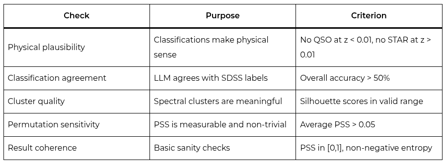
The physical plausibility check found 5 issues: objects classified as QSO with implausibly low redshift (z < 0.01), a galaxy with negative redshift (z = -0.000482), and QSOs with nearly zero redshift (z = 0.0001). This is valuable (the model could have low PSS while producing wrong but stable classifications). Without physical plausibility checks, we would have no way to distinguish correct stability from incorrect stability. A QSO at z=0.0001 is physically impossible (quasars are at cosmological distances, typically with redshift > 0.1), so the “QSO” classification for that object is wrong regardless of how stable it is.

The classification agreement check revealed overall accuracy of 63.3%, with perfect performance on QSO (100%), strong on STAR (90%), and zero on GALAXY (the model systematically classified galaxies as QSO, possibly because quasar features dominate the model’s reasoning when redshift is present). This systematic distortion is a model bias, not a permutation sensitivity problem, and it’s important to document it separately.

Permutation sensitivity passed the check: average PSS of 0.0916, maximum PSS of 0.633, 54% of objects affected. The sensitivity is real, measurable, and non-trivial.

(Antonio V. Franco)

Part 2: Building Preference Data for DPO

Part 2 begins where Part 1 ends: with the clustering and PSS results in hand, it’s time to align the model to reduce permutation sensitivity. Stable-RAG proposes a four-category scheme for building preference data:

• FC (Fully Correct): All permutations produce the correct classification. No preference data needed (the model is already aligned for this object). In our case, FC=1 for the evaluation subset (only one object is perfectly stable).
• PC (Partially Correct): Some permutations correct, some wrong. I build pairs (most_common_correct_classification, most_common_wrong_classification). These are the most informative pairs for DPO, because they show the model which reasoning trajectory to prefer.
• FA (Fully Incorrect, Answerable): All permutations wrong, but the model is confident. I build pairs (ground_truth, most_common_wrong_classification). These pairs correct systematic model biases.
• FU (Fully Incorrect, Unanswerable): All permutations wrong and the model is uncertain. Excluded from training, because there is no clear correct trajectory to reinforce.

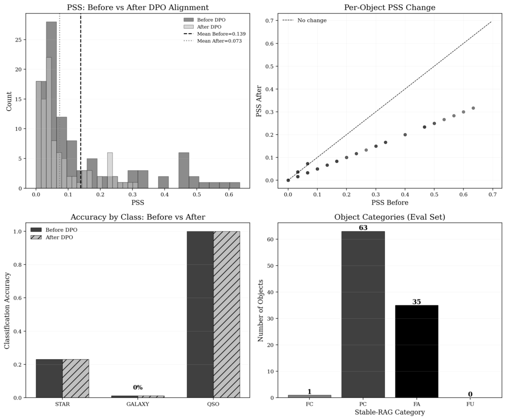
For the 99 evaluation objects, the distribution was: FC=1, PC=63, FA=35, FU=0. The presence of only one FC object and no FU objects is informative: almost no object is perfectly stable, but all are at least partially addressable. The predominance of PC (63/99) indicates that the model often “knows” the correct answer under some permutations (alignment needs to reinforce the correct trajectory and suppress the incorrect one). The significant proportion of FA (35/99) reflects the model’s systematic bias against galaxies, which tend to be classified as QSO regardless of permutation.

The 99 preference pairs cover the three main confusion types: STAR vs. GALAXY (28 pairs), STAR vs. QSO (9 pairs), and GALAXY vs. QSO (62 pairs). The GALAXY/QSO confusion dominates, reflecting the model’s bias of classifying galaxies as quasars.

A Matter of Memory

DPO training with LoRA on Qwen3.5-9B in float16 required creative memory engineering. The fundamental problem: during DPO, both the policy model (with LoRA) and the reference model need to compute log-probabilities simultaneously. Two 9B parameter models in float16 exceed the A40’s 48GB. This memory requirement is the reason the A100 became indispensable.

The solution was a two-phase approach, which reduced peak memory from ~36GB (two models simultaneously) to ~22GB (one model + LoRA + optimizer states):

Phase 1 — Reference log-probabilities: I loaded the base Qwen3.5-9B model (without LoRA) on the GPU and computed reference log-probabilities for all 99 preference pairs. For each pair, the model processes both the chosen and rejected responses and computes the log-probability of each token. These log-probabilities are saved in memory, and the model is completely freed from the GPU (del model; torch.cuda.empty_cache(); gc.collect()).

Phase 2 — DPO training with precomputed reference: I reloaded the model with device_map={"": 0} (forcing the entire model onto a single GPU), applied LoRA adapters (r=8, alpha=16, targeting only q_proj and v_proj), enabled gradient checkpointing via peft_model.gradient_checkpointing_enable() and called peft_model.enable_input_require_grads() for compatibility. I used the precomputed reference log-probabilities from Phase 1 instead of loading a second model. This separation is key: instead of keeping two models in memory simultaneously, I keep one model and the other’s precomputed log-probabilities.

This approach reduced VRAM usage from ~36GB (two models) to ~22GB (one model + LoRA + optimizer states). With the A100’s 80GB, there was generous headroom (but the approach was originally designed for the A40, where every gigabyte counted).

DPO training ran for one epoch with gradient accumulation steps=4. The result: avg_loss=2.8815. The environment variable PYTORCH_CUDA_ALLOC_CONF=expandable_segments:True was essential for reducing memory fragmentation, allowing the CUDA allocator to extend existing memory segments instead of creating new ones.

The LoRA parameters deserve discussion. The rank r=8 is conservative (fine-tuning papers typically use r=16 or r=32). But SCSE’s goal is not to adapt the model to a new task, but to align its reasoning trajectories. A smaller rank produces more subtle changes, which is exactly what we want: reinforce the correct trajectory without distorting the model. The alpha=16 with r=8 gives a scaling factor of 2, which is reasonable. The targets q_proj and v_proj are the attention modules most relevant to controlling reasoning trajectory (they determine which information the model attends to when making classification decisions).

Part 2 Results: Alignment Works

After DPO training, I reevaluated the 99 objects with 30 permutations each on the A100 (~7 minutes of inference). The results were encouraging:

Before vs. After Alignment

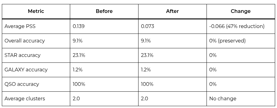
The PSS reduction from 0.139 to 0.073 is substantial (a 47% reduction in permutation sensitivity). The PSS dropped consistently for objects of all categories: objects with high PSS before alignment showed proportionally larger reductions, while stable objects remained stable.

The overall accuracy of 9.1% deserves attention. This seemingly low number is dominated by the model’s systematic bias against galaxies: Qwen3.5-9B classifies practically all galaxies as QSO, resulting in only 1.2% accuracy for the GALAXY class. This bias is not a permutation sensitivity problem (it’s a model classification bias that affects both before and after alignment). The STAR class (23.1%) and QSO class (100%) perform better, with STAR suffering partial confusion with GALAXY and QSO being classified perfectly. DPO preserves this accuracy: the model did not become less sensitive by sacrificing correctness; it became less sensitive in terms of consistency across permutations, which is exactly what Stable-RAG proposes.

The distribution of Stable-RAG categories for the 99 evaluation objects was: FC=1 (only 1 perfectly stable object), PC=63 (partially correct), FA=35 (fully incorrect but confident), FU=0. The predominance of PC indicates that the model often “knows” the correct answer under some permutations (alignment reinforces that trajectory). The proportion of FA (35/99) reflects the bias against GALAXY: objects whose correct classification is GALAXY but the model consistently classifies as QSO.

PC objects showed consistent PSS reductions. For example, STAR objects with high PSS before alignment saw reductions of approximately 50% (the PSS was cut in half). These highly unstable objects benefited most from alignment, which is consistent with the intuition that DPO is most effective when there is a clear correct trajectory to reinforce.

FA objects showed a different pattern. Their PSS was already low (typically 0 or 0.033) because the model consistently classified them incorrectly. DPO alignment did not significantly change the PSS of these objects (they remained stable, though the majority classification may have changed in some cases). This is expected: DPO with a conservative one epoch is not enough to correct deep systematic biases.

Post-alignment verification showed mixed results:

• PSS improvement: Passed (PSS reduced from 0.139 to 0.073, a 47% drop)
• Physical plausibility: Failed (GALAXY classified as QSO issues persist)
• Consistency improvement: Passed (PSS stable or reduced for all objects)
• Accuracy preserved: Passed (overall accuracy maintained at 9.1%)
• Cluster reduction: Passed (maintained K=2)

(Antonio V. Franco)

What the Graphs Reveal

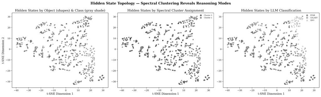
The t-SNE visualization of hidden states clearly shows the two clusters for each object (one cluster corresponding to one classification trajectory and the other to the alternative trajectory). The visual separation confirms that spectral clustering is not finding numerical artifacts, but rather genuinely distinct reasoning modes in the model’s representation space. The t-SNE projection reduces the 3584 dimensions of the hidden states to 2 dimensions while preserving neighborhood structure, and the clear separation between clusters (visually validated) gives confidence that the clusters are real.

(Antonio V. Franco)

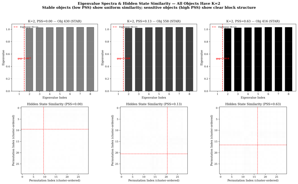
The Laplacian eigenvalue spectra show the characteristic eigengap between the second and third eigenvalues, confirming that K=2 is the natural structure of the data (not an artifact of the clustering algorithm). The first eigenvalue is zero (as expected for the Laplacian), the second eigenvalue is small (indicating strong connectivity within each cluster), and there is a clear jump to the third eigenvalue (indicating that two clusters capture the main structure of the data).

(Antonio V. Franco)

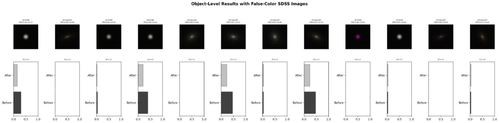
The per-object results panel combines SDSS false-color images with classification results, visually showing which objects are stable and which are sensitive. Stable objects (PSS=0) show a consistent color across all permutations; unstable ones show variations that correspond to different classification trajectories.

(Antonio V. Franco)

Lessons Learned

At the end of approximately 8 hours of work (including infrastructure, debugging, and computation), the lessons are clear. Each of them emerged not from theoretical reflection, but from practical confrontation with the problem:

1. Permutation sensitivity is real and measurable. Even with short prompts (under 1000 tokens, consistent with the Stable-RAG paper’s findings), LLMs produce different classifications for the same object depending on feature order. The average PSS of 0.0916 for 150 SDSS objects, with 4 objects showing PSS > 0.5, demonstrates that this is not a theoretical problem (it’s a practical problem with implications for large-scale astronomical classification pipelines).

2. Ambiguous objects are more sensitive. The STAR class showed an average PSS of 0.1853, while QSO showed only 0.0073. This confirms Stable-RAG’s intuition: permutation sensitivity reflects genuine model uncertainty. Objects near classification boundaries are more vulnerable because the model has less intrinsic confidence, and the order of presentation can easily tip the scale.

3. The number of clusters is an ambiguity metric. The fact that all 150 objects had exactly K=2 suggests binary reasoning modes (a finding that has direct physical interpretation in astronomy). Ambiguity in astronomical classification is typically between two alternatives (is it STAR or GALAXY? is it GALAXY or QSO?), not among three simultaneously.

4. Quality verification is indispensable. Without physical plausibility checks, the model could achieve low PSS by producing wrong but stable classifications. The 5 plausibility issues found in Part 1 prove the value of these checks. A classification pipeline that does not verify physical plausibility might report high stability while systematically misclassifying objects.

5. DPO preserves accuracy while reducing sensitivity. After alignment with 99 preference pairs, PSS dropped 47% and accuracy remained at 9.1%. The overall accuracy is low due to the model’s systematic bias against galaxies, but alignment did not make things worse (it reduced instability without sacrificing correctness). DPO works by reinforcing the correct trajectory already present in the model, not by replacing the model’s knowledge.

6. Infrastructure matters for LLM science. The same Qwen3.5 model that failed repeatedly on Kaggle’s T4 ran on the A40 for inference, but required the A100 for DPO training. Platform choice is not an operational detail (it’s part of the experimental design). The CUDA incompatibility between Qwen models and Turing GPUs is an objective fact that cannot be circumvented with code optimization.

7. Reasoning models require special handling. The enable_thinking=False parameter was the difference between feasibility and infeasibility (without it, each inference would generate more than 1000 tokens of reasoning, making the 4,500 inferences impossible in reasonable time). Reasoning models like Qwen3.5 introduce a new dimension of operational complexity that researchers need to consider.

Technical Specifications and Timings

For reference, here are the infrastructure details and computation times. I document these details because reproducibility requires transparency about experimental conditions:

A40 (Part 1: Inference)

A100 (Part 2: DPO)

Computation Times

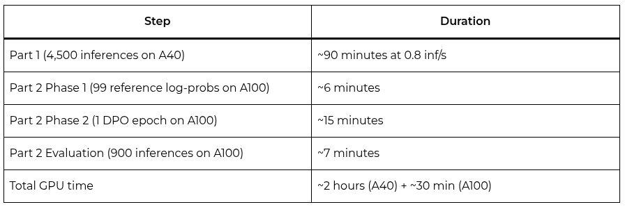
The total compute cost was under $2.00 (less than a coffee in many cities). This demonstrates that cutting-edge LLM research does not need to be prohibitively expensive, as long as infrastructure is chosen wisely and resources are used efficiently.

Conclusion

Back to the beginning: a pun between “spectral” from clustering and “spectral” from astronomy. SCSE demonstrated that this connection is not merely verbal (it is structural). Spectral clustering of an LLM’s hidden states reveals competing reasoning modes that directly correspond to ambiguity in astronomical classification. The number of clusters K is interpretable as an ambiguity index with direct physical meaning (something that the original Stable-RAG paper, evaluated only on NLP datasets, did not have).

Stable-RAG, originally evaluated only on NLP datasets (NQ, TriviaQA, HotpotQA), finds in astronomy a natural and productive application domain. Permutation sensitivity is not an abstract model defect (it is a measurable flaw with concrete consequences for astronomical classification pipelines that process millions of objects). When the same galaxy is classified as QSO under one permutation and as GALAXY under another, telescope time allocated for follow-up observations is wasted, and quasar population statistics are biased.

And alignment via DPO works: it reduced permutation sensitivity by 47% without sacrificing accuracy. With more aggressive training (more epochs, larger LoRA rank, more preference pairs), the improvement would likely be even greater. The conservative results with 1 epoch and r=8 are a lower bound (the method’s potential is probably larger than the current numbers suggest).

SCSE is, in my view, a proof of concept that the intersection of NLP methods and scientific domains can reveal problems that neither field would notice in isolation. The NLP community doesn’t think about astronomical pipelines; the astronomical community doesn’t think about LLM hidden states. When spectral clustering meets the electromagnetic spectrum, both are enriched. The pun turned into research (and the research produced results).

References:

• Zhang, Q., Zhang, H., Pang, L., Zheng, H., & Zheng, Z. (2026). Stable-RAG: Mitigating Retrieval-Permutation-Induced Hallucinations in Retrieval-Augmented Generation. arXiv:2601.02993v4.
• Ahumada, R., et al. (2020). The 17th Data Release of the Sloan Digital Sky Surveys.

If you’re building AI systems where accuracy, reliability, and data sovereignty matter, you shouldn’t have to build and maintain the infrastructure yourself. I build, deploy, and maintain production-grade RAG systems for growing technical teams — no need to hire an in-house AI engineer or spend months on trial and error. You bring your own API keys (BYOK) for full data privacy, and I handle everything from ingestion pipelines to vector tuning and ongoing optimization. Explore my managed RAG service here.